A Reinforcement Learning agent figures out how to Control Floquet-Engineered Quantum States in a numerical simulation of a quantum experiment. The ability of RL to control systems far away from equilibrium is demonstrated by steering the quantum Kapitza oscillator into the stabilized inverted position in the presence of a strong periodic drive.
In order to build intuition about the problem, we first introduce the classical Kapitza pendulum, and then discuss the quantum Kapitza oscillator. Check out this paper for a more detailed and complete discussion [1].
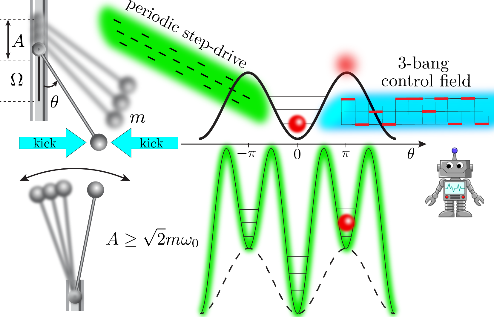
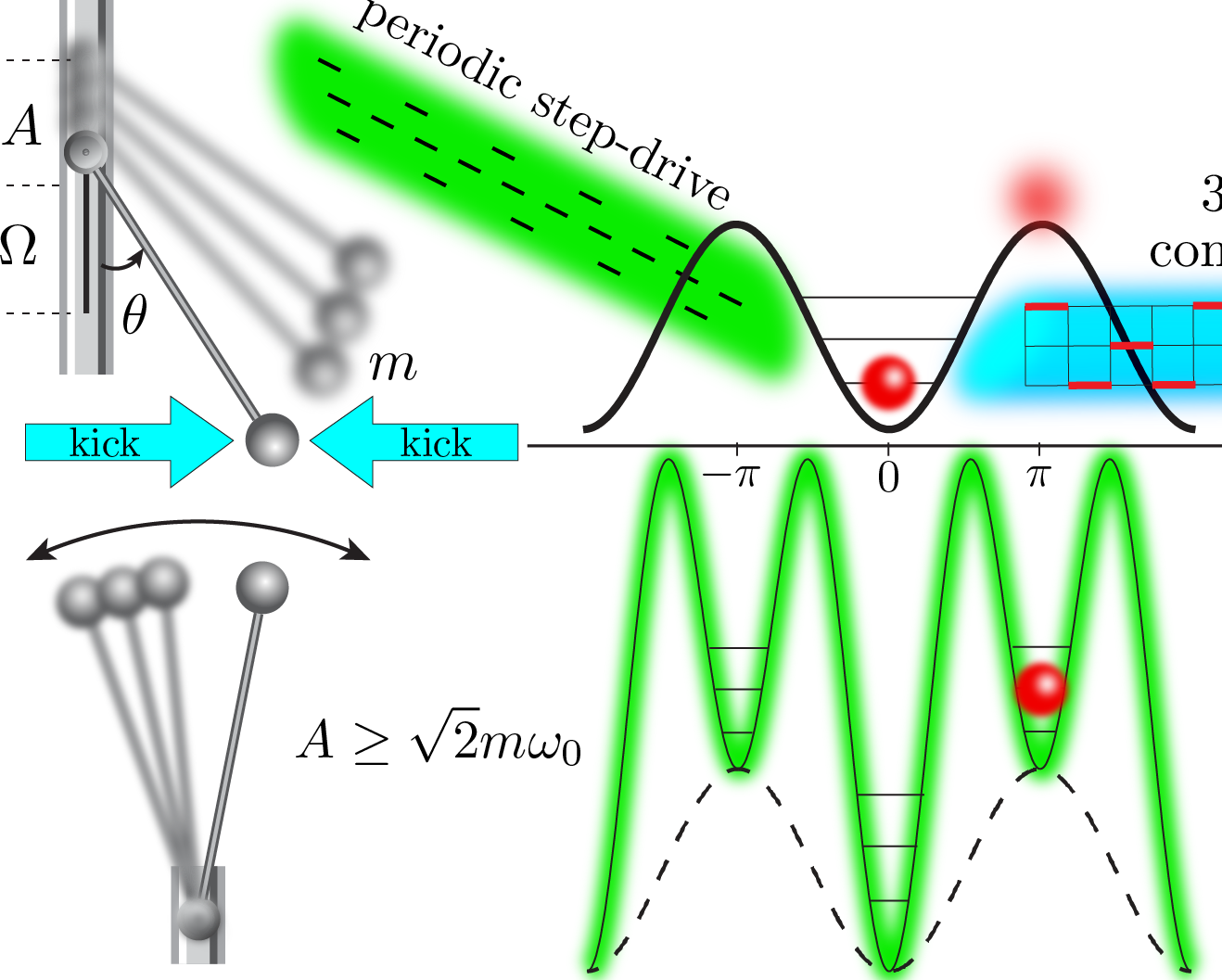
The classical Kapitza oscillator (scroll down for the quantum version) is a pendulum like the one shown on the figure above. The motion of the pendulum is described by the angle trajectory \(\theta(t)\) w.r.t. the vertical axis. Recall that such a pendulum has a stable equilibrium point at \(\theta=0\), and a metastable equilibrium at the inverted position \(\theta=\pi\). This metastable equilibrium is unstable for all practical purposes: any small perturbation will cause the pendulum to tip over. Kapitza (and probably others before him) figured out that a high-frequency periodic modulation of the pendulum pivot point has a stabilizing effect on the unstable equilibrium \(\theta=\pi\), above a critical value for the driving frequency [2] . To see how this works in practice, see this video.
|
Optimal protocol found by the RL agent to prepare the inverted position state in the classical Kapitza pendulum [1]. Turning off the control field but keeping the periodic drive on, the pendulum oscillates about the stabilized equilibrium at the inverted position. When the periodic drive is turned off, the pendulum tips over. |
The pendulum is taken away from equilibrium by the strong periodic drive, which also changes its stability properties. The equations of motion for the Kapitza pendulum admit no closed-form solution. Controlling the system on top of the strong periodic drive to reach the target state at the inverted position starting from the stable equilibrium \(\theta=0\) is an intriguing challenge. The video above shows the solution found by our Reinforcement Learning agent after a series of attempts (click here for a detailed movie legend.).
 Reinforcement Learning (RL) is a branch of Machine Learning (ML), in which an agent learns to find the optimal policy to perform a specific task, based on feedback as a result of interaction with its environment [3]. The theory behind RL is built on Markov decision processes: the agent finds its environment in a given state, and is presented with a choice of actions to pick, each of which changes the state of the environment.
As a consequence of its decision, the agent is given a reward, depending on the new environment state. Similar to animals being rewarded for achieving the task during training, the goal is to maximize the long-time expected return. This is accomplished through learning about those properties of the environment which are particularly relevant for maximizing the reward. In doing so, the algorithm autonomously figures out an optimal policy to perform the task [see Fig. on the right].
Reinforcement Learning (RL) is a branch of Machine Learning (ML), in which an agent learns to find the optimal policy to perform a specific task, based on feedback as a result of interaction with its environment [3]. The theory behind RL is built on Markov decision processes: the agent finds its environment in a given state, and is presented with a choice of actions to pick, each of which changes the state of the environment.
As a consequence of its decision, the agent is given a reward, depending on the new environment state. Similar to animals being rewarded for achieving the task during training, the goal is to maximize the long-time expected return. This is accomplished through learning about those properties of the environment which are particularly relevant for maximizing the reward. In doing so, the algorithm autonomously figures out an optimal policy to perform the task [see Fig. on the right].
To control the pendulum, the RL agent constructs protocols \(h(t)\) of fixed length: sequences of \(120\) short horizontal kicks exterted on the pendulum, shown by the arrows in the figure and movie above. The kicks come in \(3\) types, and can point left, right, or there can be no kick at all (see \(3\)-bang control fleid shown in cyan in the figure above). Each time step, the RL agent has to choose the best kick type, according to its gathered knowledge [for the experts, we use Q-Learning [3]]. The control protocols have a finite duration \(t_f\). In total, there are \(3^{120}\approx 10^{57}\) possible protocols configurations - more than there are atoms in the universe. The agent is stimulated to look for better protocols by receiving a reward, depending on the pendulum position in the end of every protocol and the pendulum final momentum \(p_\theta\) (we don’t want the pendulum to overshoot):
\[r(\theta,p_\theta) = \frac{1}{\pi^2}\left[ (\theta(t_f)+\pi)\mathrm{mod}(2\pi) - \pi \right]^2 - 4\vert p_\theta(t_f)\vert^2,\qquad r\in[-\infty ,1].\]The reward is given only once, at the end of the protocol. Hence, with no knowledge about the controlled system, our RL agent progressively learns how it behaves and uses this information to prepare the inverted state (see movie above).
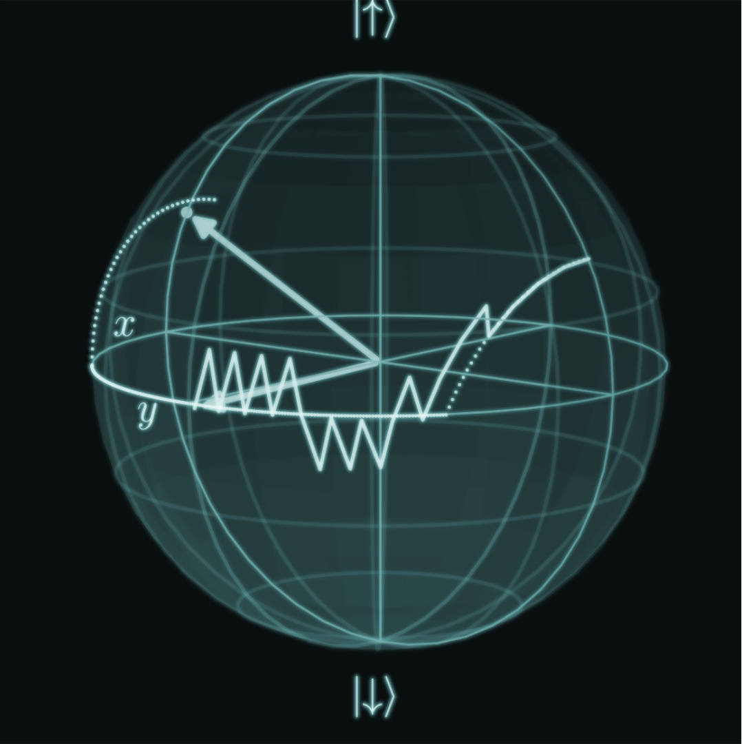
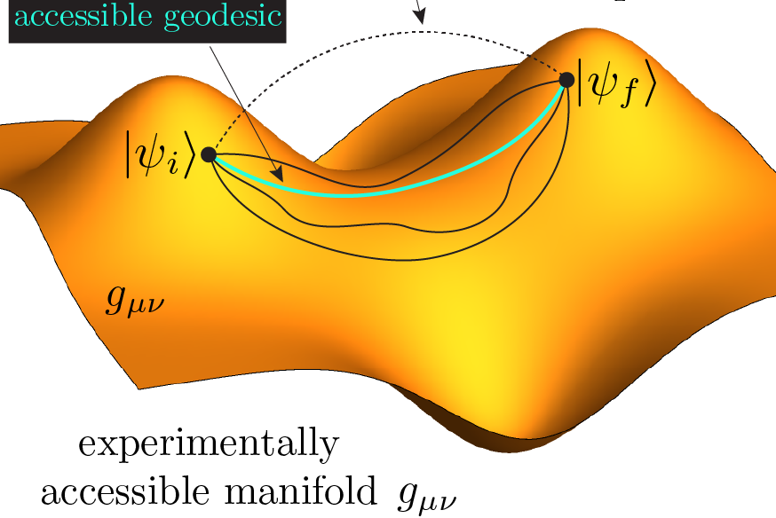
Now that we have built some intuition about the physics of the controlled system, we introduce the quantum version of the pendulum. In Quantum Mechanics, the state of the quantum Kapitza oscillator is described by a wavefunction \(\vert\psi(t)\rangle\), which contains all information about the oscillator. A significant challenge for autonomous quantum control arises from the lack of access to the quantum states which are unmeasurable mathematical constructs. Even though one cannot measure the quantum state in experiments, there is a way to interactively learn how to steer the system during its evolution. Using the determnistic character of the Schrödinger equation, starting from a fixed initial quantum state \(\vert\psi_i\rangle\), one can parametrize the accessible states at later times \(\vert\psi(t)\rangle\) by the protocol sequence \(h(t)\) up to time \(t\) [1]. Whereas quantum states cannot be measured, the applied protocols \(h(t)\) can actually be kept track of. Hence, fixing the initial state, one can infer which state the quantum system ought to be in at a later time, from the applied protocol. In fact, the minimal amount of information an autonomous agent can have about the controlled quantum system is the applied protocol sequences.
Another challenge in experiments is the nondeterministic character of projective quantum measurements. Since they destroy the state, one is allowed to measure only once, at the end of the protocol when the system has evolved into the state \(\vert\psi(t_f)\rangle\). Projective quantum measurements are modeled to return \(1\) with probability set by \(F_h(t_f)=\vert\langle\psi(t_f)\vert\psi_\ast\rangle\vert^2\) (also known as fidelity) if the system is found in the target state \(\vert\psi_\ast\rangle\), and \(0\) otherwise. Therefore, the algorithm seeks to maximize the fidelity \(F_h(t_f)\), whose true value remains unknown at the time of measurement, and is only estimated from the data. The estimate of the fidelity at the end of the protocol \(t_f\) is given as a reward to the RL agent:
\[r(\vert\psi(t_f)\rangle) = \mathrm{estimate\ of}\left(\vert\langle\psi(t_f)\vert\psi_\ast\rangle\vert^2 \right).\]During the learning process, the situation is in fact much more complicated: as the available protocol family is explored, the true probability \(F_h(t_f)\) to determine the measurement, changes from one protocol to the next, as different protocols in general lead to different final states.
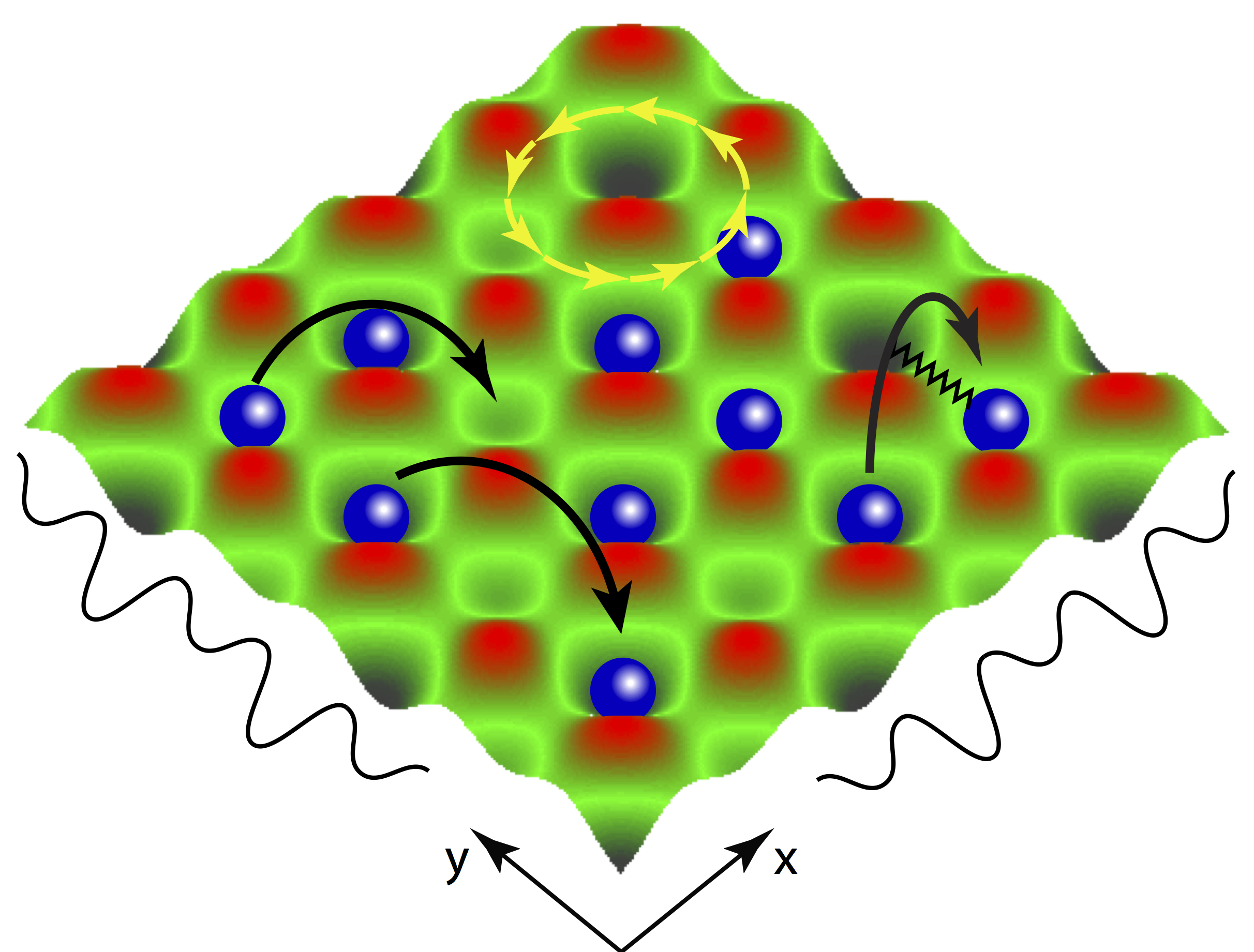
The best protocol found by the RL agent to control the quantum Kapizta oscillator is shown below. To visuallize the state, we show its real-space probability distribution \(\vert\langle\theta\vert\psi(t)\rangle\vert^2\). The circle below represents the \(\theta\)-space and the color of the boxes - the probability to find the oscillator in the corresponding angle sector. Unlike classical states, the quantum state is delocalized – it occupies simultaneously all possible \(\theta\)-values but with different probabilities (see colorbar). The RL agent figures out how to bring the distribution at the inverted position with fidelity \(\sim 89.8\%\) in a sequence of attempts in the presence of the drive (the maximal possible fidelity value is not known for this setup). The movie below shows the final result (click here for a detailed movie legend.).
|
Optimal protocol found by the RL agent to prepare the inverted position Floquet eigenstate in the quantum Kapitza oscillator [1]. Turning off the control field but keeping the periodic drive on, the oscillator state remains trapped about the stabilized equilibrium at the inverted position. Unlike the classical pendulum, quantum effects do not allow the oscillator wavefunction to tip over even when the drive is turned off. |
For more details on the RL learning procedure, check out the entire paper.
References:
[1] M.B., Phys. Rev. B 98 224305 (2018).
[2] P. L. Kapitza, Soviet Phys. JETP, 21 588–592, (1951).
[3] R. S. Sutton and A. G. Barto, Reinforcement Learning: An Introduction (MIT Press, Cambridge, MA, 2017).
[4] M.B., A. G.R. Day, D. Sels, P. Weinberg, A. Polkovnikov, and P. Mehta, Phys. Rev. X 8 031086 (2018).
Copyright © 2018 Marin Bukov