Introduction to Deep Reinforcement Learning
FINAL GRADES: enter the password and click here
Final Presentation/Exam Schedule: attendance is mandatory for all members of the presenting team only; all other students are welcome to attend!
| Team # | Presentation Title | Date | Time | Project |
|---|---|---|---|---|
| 14 | Comparing the performance of Dueling Network Architectures for Deep Reinforcement Learning with older models | 3/2 | 5:15pm | |
| 4 | Alpha Ideas in Algorithmic High-Frequency Trading | 4/2 | 5:15pm | |
| 6 | Zermelo’s problem: Optimal point-to-point navigation in 2D turbulent flows using Reinforcement Learning | 5/2 | 4:30pm | |
| 11 | Resource Management with Deep Reinforcement Learning | 5/2 | 5:15pm | |
| 1 | Solving the Rubik’s Cube with Deep Reinforcement Learning | 8/2 | 4:30pm | |
| 3 | Solving the Rubik’s Cube with Deep Reinforcement Learning | 9/2 | 4:30pm | |
| 10 | Spacecraft maneuvering near small bodies using reinforcement learning | 10/2 | 4:30pm | |
| 5 | Playing and Experimenting on Atari Games with Deep Reinforcement Learning | 11/2 | 4:30pm | |
| 2 | Using Reinforcement Learning to Sustain High-density Populations in Conway’s Game of Life | 11/2 | 5:15pm | |
| 13 | Snake Game using Deep Reinforcement Learning | 12/2 | 4:30pm | |
| 8 | Indian Crossroads Traffic Warden | 12/2 | 5:15pm |
offered: Winter Semester 2020/21
instructor: Marin Bukov, PhD
lectures: Sat, 1 pm - 4 pm, ONLINE
coding session: Fri, 6 pm - 8 pm, ONLINE
credits: 6 ECTS
exam: written project (see below)
office hours: by appointment
latest reading material: click here
Lecture Notes:
-
16/1: lecture notes: Continuous Actions: Policy Gradients with (un)bounded continuous actions (Gaussian and Beta distributed policies), Q-learning with continuous actions: Deep Deterministic Policy Gradient (DDPG)
-
9/1: lecture notes: Advanced Policy Gradients: Natural Policy Gradient, Trust Region Policy Optimization (TRPO), Proximal Policy Optimization (PPO), Entropy-based Exploration
-
19/12: lecture notes: Deep Q-Learning: fitted Q-iteration, deep online Q-learning, DQN, replay buffer, target network, deep double Q-learning
-
12/12: lecture notes: Actor Critic Methods: online and offline actor critic algorithms
-
5/12: lecture notes: Deep Policy Gradient: REINFORCE algorithm, high variance problem, baselines, practical implementation
- 28/11: lecture notes: Basics of Deep Learning: Linear and logistic regression, fully-connected and convolutional neural networks
-
21/11: lecture notes: Gradient Descent Algorithms: SGD, SGD with momentum, NAG, RMSProp, Adam
-
14/11: lecture notes: Temporal Difference Learning: SARSA, Q-Learning, Expected SARSA, Double Learning
-
7/11: lecture notes: Monte Carlo Methods for RL: First-visit MC, MC with Exploring Starts, Importance Sampling
-
31/10: lecture notes: Dynamic Programming: Policy Evaluation, Policy Iteration, Value Iteration, Policy Improvement
-
24/10: lecture notes: Agent-Environment Interface: Episodic and Non-episodic Tasks, Value and Action-Value functions, Policies, Optimal Policy and Optimal Value Functions, Bellman Equation
-
17/10: lecture notes: Gaussian mixture models, Markov processes, Ising models, Monte Carlo sampling
- 10/10: logistics slides
Coding Session Notebooks:
-
15/1: Q/A session
-
8/1: Notebook 10: Deep Actor-Critic Methods in JAX: ipynb, pdf, html
-
11/12: Notebook 8: Deep Policy Gradient in JAX: ipynb, pdf, html
-
27/11: Notebook 6: Gradient Descent Methods: ipynb, pdf, html
-
20/11: Notebook 5: Temporal Difference Learning: ipynb, pdf, html
-
13/11: Notebook 4: Monte Carlo Methods for RL: ipynb, pdf, html
Instructions and \(\LaTeX\) templates for the final project:
- project proposal: template / instructions
- final project: template / instructions
- peer review: instructions
- final presentation instructions
Python libraries setup:
-
(unless you already have it) create a Google account; it will give you access to Google Colab, and other features. You don’t need to use gmail; you can also delete the account once the semester is over, in ase you don’t want to keep it.
-
check out Google Colab; it allows you to train models on a GPU/TPU for up to 12 hours. Read carefully the FAQs. Google Colab has python, and all of the packages listed below, built in, so you may choose not to do the following steps.
-
(unless you already have it) install Python 3. We recommend using the Anaconda package manager; read the getting started with conda page
-
(unless you already have it) install scipy and numpy (anaconda provides the MKL-optimized numpy version by default). If you have conda installed, this is as easy as opening up the conda terminal and typing:
conda install numpy scipy -
(unless you already have it) install Jupyter notebook:
conda install -c anaconda jupyter. To make the conda environment appear as a kernel in Jupyter notebooks, doconda install ipykernel, followed bypython -m ipykernel install --user --name RL_course --display-name "RL_course". -
(unless you already have it) install JAX. Before you do so, you will need
pip:conda install pip
Course Description
Alongside Supervised and Unsupervised Learning, Reinforcement Learning (RL) is a branch of Machine Learning (ML), in which an agent learns to find the optimal strategy to perform a specific task, based on feedback as a result of interaction with its environment.
The ground-breaking success of RL lead to significant recent advances in Artificial Intelligence: DeepMind’s RL agents play video and board games using only information from pixels of the screen/photo of the board, defeating human champions. RL algorithms are now widely used in ML, robotic training, biochemistry, and physics, and have increasing applications in industry: e.g., an RL agent recently managed to reduce Google’s Data Center cooling bill by 40%.
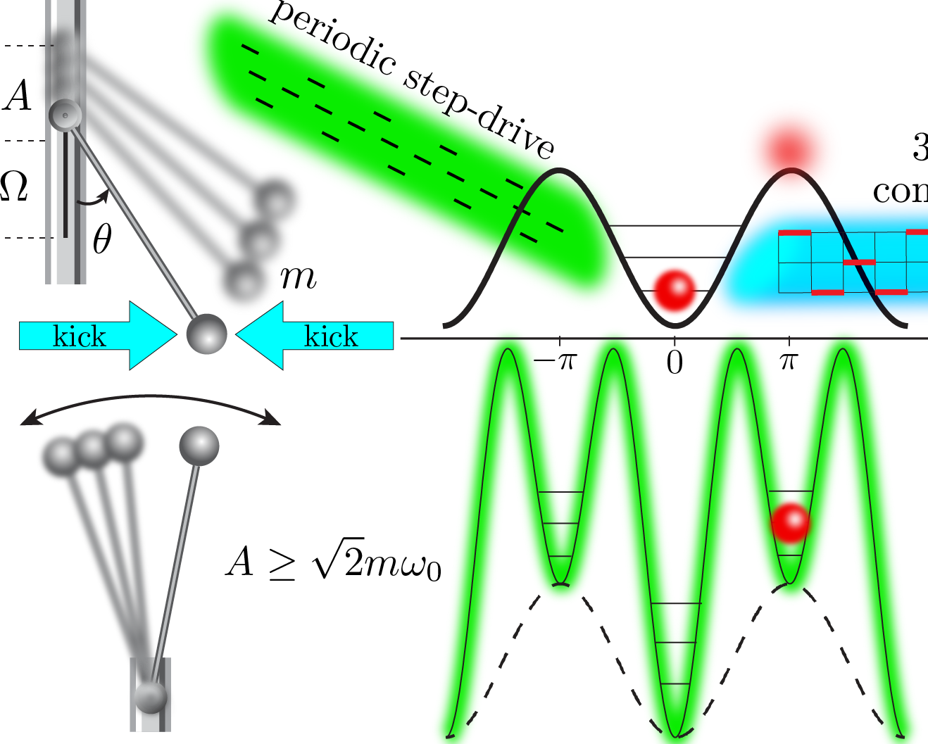
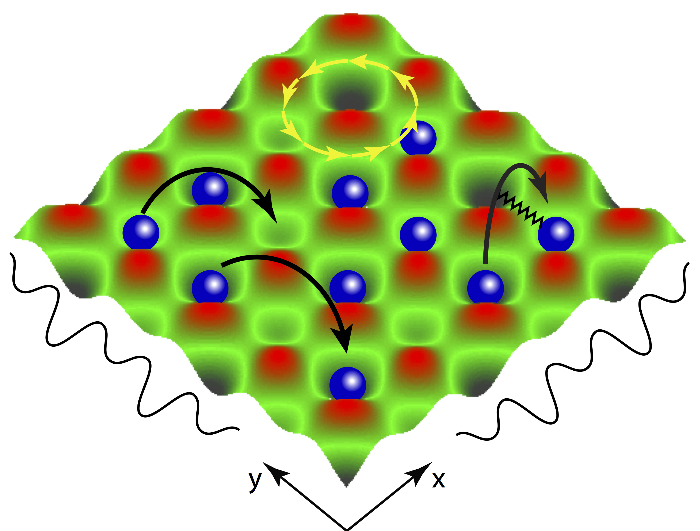
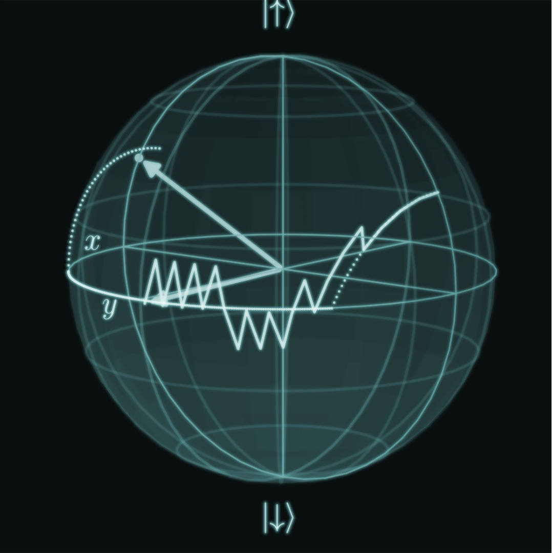
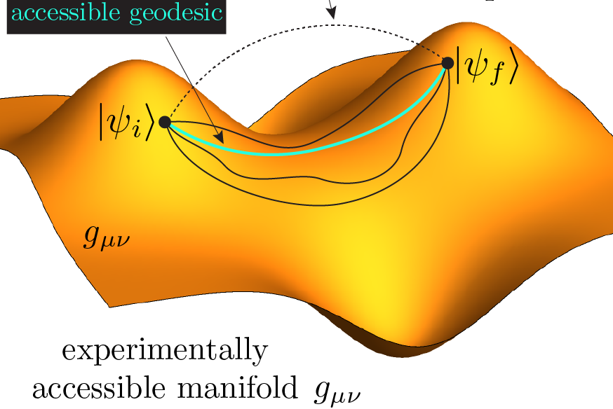
Recently, Reinforcement Learning ideas have been applied in the study of fundamental science, including classical and quantum physics: RL agents can successfully navigate turbulent flows, prepare the states of quantum bits (qubits), identify noise-robust quantum channels required for quantum computing, and explore the vast space of string vacua, just to name a few.
This special lecture course provides an introduction to Deep Reinforcement Learning (cf. syllabus below). The class is suitable for PhD students, master students, and advanced bachelor students (3rd and 4th year). We will discuss the theory and basic principles behind RL, and apply them in practice to study their various applications in physics, computer science, and optimal control.
For interested students, we also offer a student seminar worth 3 ECTS.
Prereqs
-
math prerequisites: linear algebra, analysis in many variables, basic concepts of probability theory. Proficiency in deep learning is not required but can be very useful.
-
physics prerequisites: not required, but general physics, basic statistical physics and basic quantum mechanics knowledge will be helpful for understanding some examples we will discuss.
-
programming prerequisites: experience with Python or a similar programming language. Python will be used during the discussion sections. Familiarity with JAX, TensorFlow, PyTorch, or another machine learning library is not required in advance, but can greatly facilitate learning the course material. The Google JAX library will be used in the discussion sections.
-
language: the lecture course and the coding sections will be held exclusively in English, but students will also be allowed to ask questions in Bulgarian. For the final written project and its presentation, students are allowed to use either English or Bulgarian. A bonus is added to the final grade if English is used by a student exclusively throughout the course.
Syllabus
| 1. Review of selected concepts of probability theory: Markov processes, Gaussian mixture models, Monte Carlo sampling |
| 2. Basics of Reinforcement Learning (RL): RL as a Markov decision process: states, actions and rewards. Strategy/Policy. Value function and action-value (Q-) function. Exploration-Exploitation dilemma |
| 3. Dynamic Programming: policy evaluation, policy improvement (Bellman’s optimality equation), policy iteration, value iteration |
| 4. Tabular RL algorithms. Temporal Difference (TD) learning: SARSA, Q-Learning, Double learning |
| 5. Deep Learning in a Nutshell: Gradient Descent Algorithms, Linear and Logistic Regression, Deep Neural Networks |
| 6. RL algorithms with Function Approximation: Policy Gradient and the REINFORCE algorithm |
| 7. Deep Reinforcement Learning algorithms: Imitation Learning, Deep Policy Gradient, Deep RL with Q-functions, etc. |
| 8. Advanced topics (time permitting): Improving exploration, RL with continuous actions, RL and its relation to Bayesian Inference, RL and its relation to statistical physics |
| 9. Open problems at the interface of physics and RL (time permitting) |
Literature / Materials
-
Sutton and Barto, Reinforcement Learning: an Introduction, 2nd Ed., MIT Press, 2018
-
YouTube lecture videos of Sergey Levine’s Deep RL class at UC Berkeley
-
P. Mehta, et al., A High-Bias, Low-Variance Introduction to Machine Learning for Physicists
JAX Library
We will use JAX to code deep learning models. JAX is a python library by Google particularly suitable for automated differentiation, and with it – for deep learning research. In essence, JAX is a more pythonic version of TensorFlow, and both make use of XLA as backend. Here’s a YouTube video which introduces JAX. Check out the JAX Github repo with the installation guide. And a recent NeurIPS 2020 talk with info on TPUs.
Google Colab
You can use Google Colab free of charge for your final project. This will allow you to train models on a GPU/TPU for up to 12 hours, see the FAQs. We recommend using Google Colab for long runs of your code (instead of your local machine). Google Colab readily supports JAX. Here’s a useful 5-min read on using GPUs with Google Colab.
Final Grade
The lecture course does not contain any classic forms of written or oral examination. Final grades will be given based on a course project and its evaluation, which includes a project proposal, project completion, peer review report, and project presentation.
-
Students are required to submit a Final Project Proposal by 12:00am (midnight) on the night of Dec 5/Dec 6. The proposal lays out the problem to be studied, the RL methodology to be applied, and the expected progress timeline (Gantt chart). The Final Project Proposal counts towards the final grade. The Final Project can consist of a new numerical experiment proposed by the student or a feasible reproduction of already published results. The students can choose a topic of their own interest, after obtaining the consent of the instructor. Depending on enrollment levels in class, multiple students may be allowed to work in a team on a joint Final Project of appropriately extended scope after obtaining consent from the instructor.
-
The Final Project results are to be reported in the form of a written scientific paper, preferrably typed in LaTeX, following the criteria, guidelines, and requirements of Physical Review Letters (3700 words, double-column format, etc.). Final projects are to be submitted via email to the instructor by Jan 23, 2021 at 11:59pm (midnight) (NO exceptions!).
-
After the Final Project submission deadline, each student will participate as a reviewer in a double-blinded Peer Review process, in which they will anonymously evaluate and assess the Final Projects of other students, according to the criteria of Physical Review Letters, and submit a peer review report. The objectivity and fairness of the review reports will then be evaluated by the instructor, who serves as an editor. Peer Review counts towards the final grade for the class.
-
The ultimate evaluation of the Final Projects will be carried out independently by the instructor taking into account the students’ reports from the peer review process.
-
After the evaluation of their projects, the students are required to give a Final Project Presentation, and answer questions related to their project.
Final Grade Formation
| Task | % of Final Grade |
|---|---|
| Final project proposal (written) | 15% |
| Final project (written) | 50% |
| Peer Review reports of final projects (written) | 10% |
| Final project presentation (oral) | 25% |
| Bonus, if English is used exclusively for all of the above | 10% (extra) |
Late Submission Policy
Submitting the assignments after the deadline is strongly discouraged! However, in extraordinary circumstances, late submission may still be granted, according to the following policy: each student has a total late submission credit of 48 hours for all tasks in the course combined. Once the late submission credit has been used up, your assignment will no longer be graded and you will receive 0% for the corresponding task :( .