Control problems are optimisation tasks with the objective to find the most efficient solution satisfying given constraints. We demonstrated that the difficulty of finding the optimal solution can change abruptly, resulting in the appearance of Control Phase Transitions in the optimisation landscape.

Phases of matter, such as liquid, solid and gas, contain valuable information about the behaviour and properties of its constituents. By changing an ambient parameter, e.g. temperature or pressure, a substance can undergo a phase transition, rapidly switching from one phase to another. Understanding how phase transitions occur and behave is crucial for correctly predicting the properties and functionality of devices in harsh environments.

We uncovered the existence of genuine phase transitions in the process of preparing states in quantum systems. It is remarkable that the same laws, which govern the evaporation of water into gas, apply to optimal manipulation of quantum states – a paradigm known as spontaneous symmetry breaking. Stunningly, the state preparation problem exhibits examples of prototypical equilibrium phase transitions in classical macroscopic systems: both first and second order phase transitions, a glass phase, and symmetry breaking, see Figure. These control phase transitions, present even in low-dimensional clean quantum systems, are of non-equilibrium nature. In much the same way conventional phase transitions play a quintessential role in understanding the properties of physical substances, the quantum control phase transitions carry far-reaching consequences for manipulating quantum states.

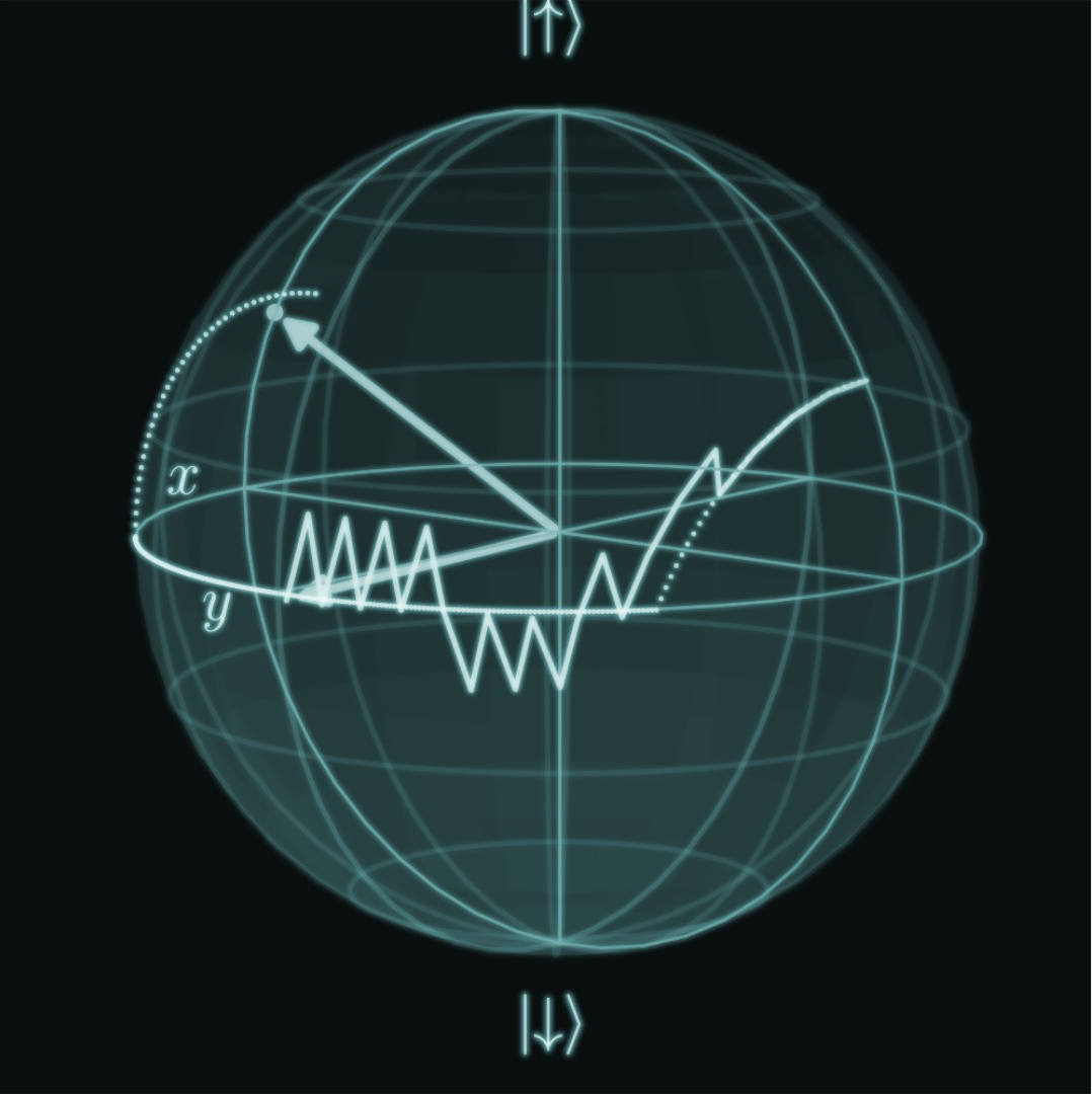
We study a two-qubit problem described by the Hamiltonian

where \(J=h_z=1\) are the interaction strength and the static magnetic field along the \(\hat z\)-axis, respectively, and \(h_x(t)\) is the time-dependent control field. The Pauli spin-\(1/2\) operators are denoted \(S^\mu_{j=1,2}\). We prepare the system at time \(t=0\) in the ground state (GS) \(\vert\psi_i\rangle\) of \(H(t)\) for \(h_{x,i}=-2\), and want to transfer the population into the target state \(\vert\psi_\ast\rangle\) – the GS for \(h_{x,\ast}=+2\) – in a fixed amount of time \(T\). Thus, our goal is to find the functional form of the driving protocol \(h_x(t)\) which maximises the fidelity of being in the target state \(F_h(T)=\vert\langle\psi(T)\vert\psi_*\rangle\vert^2\) at the end of the protocol, following Schrödinger evolution for a duration \(T\).

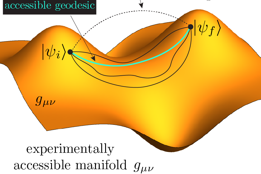
Each driving protocol induces a unique evolution of the quantum state, and thus can be classified by measuring the fidelity \(F_h(T)\) with which it prepares the target state. To every protocol, we can uniquely assign a single number – the infidelity \(I_h(T)=1-F_h(T)\) of being in the target state after evolution of time \(T\). This quantity gets smaller, the closer we get to the target state. One can imagine an infidelity landscape, which has a many local minima and maxima (“valleys” and “hills”), correspondng to different protocols. The global minimum then corresponds to the optimal protocol, which solves the optimisation problem.

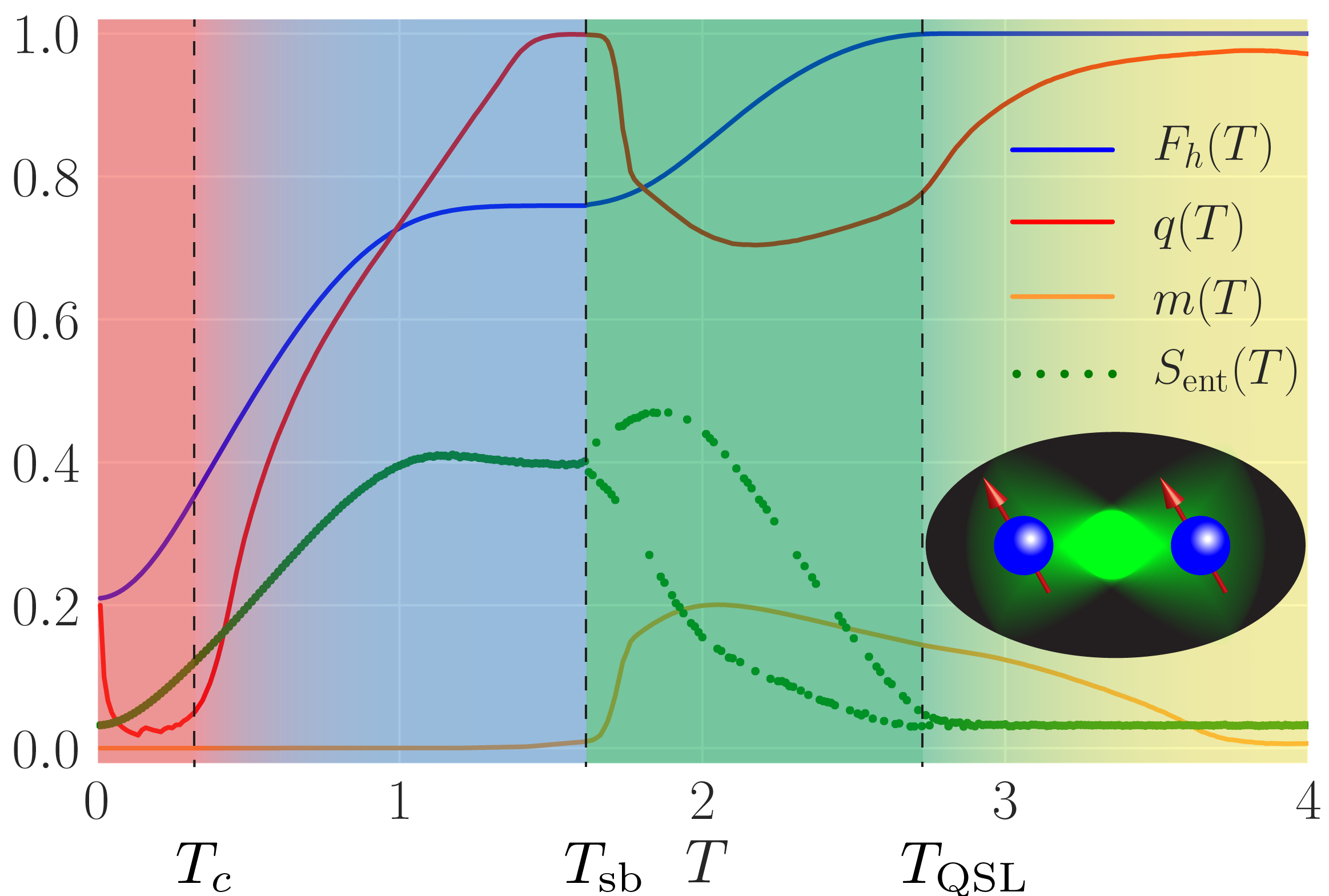
The figure above shows the phase diagram of this quantum control problem, as determined by the correlation function \(q(T)\), which measures the fluctuations between nearly optimal protocols. Starting at protocol times \(T\approx 3\), we find the optimal fidelity (blue line) at unity, which means that one can successfully and completely prepare the target state \(\vert\psi_\ast\rangle\). Therefore, the system is said to be in the controllable phase (yellow).

At the quantum speed limit critical point \(T_\mathrm{QSL}\approx 2.8\), the infidelity landscape undergoes a continuous second-order transition to a glassy phase (blue, green). This phase transition occurs in an effective classical model with non-local multi-body interactions [1]. For \(T<T_\text{QSL}\), the fidelity \(F_h(T)\) deviates from unity, and reaching the target state becomes impossible under the constraints of the problem. In this glassy phase [2], the protocols associated with local minima of the infidelity landscape become correlated, which is reflected in the finite value of the order parameter \(q(T)\). Due to the glassiness in the infidelity landscape, sophisticated algorithms with nonlocal updates are required to find the optimal protocol.

Surprisingly, the glassy phase of the system itself consists of two other phases: (i) for \(T\gtrsim T_\mathrm{sb}\approx \pi/2\), spontaneous symmetry breaking occurs in protocol space and there are two distinct, yet equivalent optimal driving protocols (green). Precisely at the symmetry breaking critical point \(T_\mathrm{sb}\), we find a discontinuity in \(q(T)\), and hence the transition is of first-order [3]. Approaching the critical point from below, we find \(q(T\to T_\mathrm{sb}^-)=1\) which means that the protocols are completely uncorrelated, while the optimal fidelity exhibits a non-analytic plateau, see Figure. On the other hand, (ii), for \(T\lesssim T_\mathrm{sb}\), the glass phase is unbroken (blue), and there exists a unique optimal protocol.

Lowering the total protocol duration \(T\) further, we encounter yet another second-order phase transition at \(T=T_c\approx 0.38\), when the various minima of the infidelity landscape coalesce into a single global minimum. This suggests that the landscape in this overconstrained phase (red) is convex, and optimisation is easy again, even though the optimal fidelities one can reach are pretty poor due to the short protocol duration.

References:
[1] A. G.R. Day, M.B., P. Weinberg, P. Mehta, and D. Sels, Phys. Rev. Lett. 122 020601 (2019).
[2] M.B., A. G.R. Day, D. Sels, P. Weinberg, A. Polkovnikov, P. Mehta, Phys. Rev. X 8 031086 (2018).
[3] M.B., A. G.R. Day, P. Weinberg, A. Polkovnikov, P. Mehta, and D. Sels, Phys. Rev. A 97, 052114 (2018).

Copyright © 2017 Marin Bukov